Spark Data Source API V2 - write query planning and execution

Before you can read anything you need to have it written in the first place. The previously considered read path is a little simpler but certainly shares a lot with the write path we'll delve into today. Initially I am going to concentrate on the basic flow and ignore predicate push-down and column pruning. As my running example I assume a trivial Spark expression that uses some existing Dataset such as "df.write.format("someDSV2").option("path", hdfsDir).save()".

A data source is represented in a logical plan by WriteToDataSourceV2 instance created by data frame writer. During planning DataSourceV2Strategy transforms the relation into a WriteToDataSourceV2Exec instance. The latter uses the Spark context to execute the plan associated with the Dataset. The resultant RDD determines the number of input partitions and so the number of required write tasks. In addition, WriteToDataSourceV2Exec helps with keeping track of WriterCommitMessages used to make writing data source partitions transactional.

Query planning

In this phase the goal is to create a WriteToDataSourceV2 from a Dataset and client-supplied options and then transform it into a WriteToDataSourceV2Exec. The process is initiated by saving a Dataset. It triggers both logical and physical planning stages.

• DataFrameWriter searches for an implementation of the DataSourceV2 marker interface. The implementation is expected to also implement the WriteSupport mixin interface that is the actual entry point into writing functionality
• WriteSupport is a factory of DataSourceV2Writer instances
• DataSourceV2Writer can create a DataWriterFactory and is ultimately responsible for committing or rolling back write partition tasks
• WriteToDataSourceV2 is the logical plan node that represents a data source
• A QueryExecution is associated with the WriteToDataSourceV2 to help with coordination of query planning
• SparkPlanner uses DataSourceV2Strategy to transform logical plan nodes into physical ones
• DataSourceV2Strategy recognizes data source logical nodes and transforms them into physical ones
• WriteToDataSourceV2 carries a DataSourceV2Writer and logical plan associated with the Dataset; both are given to WriteToDataSourceV2Exec
• WriteToDataSourceV2Exec is the physical plan node that represents a data source

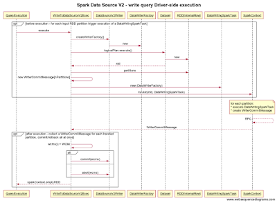
Query execution - Driver side

In this phase the goal is to obtain data partitions from the RDD associated with the Dataset and trigger execution of a write task for each partition. In this section we look at the Driver-side half of the process.

• WriteToDataSourceV2Exec creates a DataWriterFactory and a write task for each partition
• The Spark context executes the tasks on worker nodes and collects WriteCommitMessages from successfully finished ones 
• WriteToDataSourceV2Exec uses DataSourceV2Writer to commit or rollback the write transaction using collected WriteCommitMessages

Query execution - Executor side

The second half of the execution phase takes place on the Executor side. 

• DataWriterFactory is serialized to worker nodes where DataWritingSparkTask are executed
• Executor provides a DataWritingSparkTask with a Row iterator and a partition index
• The task acquires a DataWriter from the DataWriterFactory and writes all partition Rows with the DataWriter
• The task calls the DataWriter to commit writing and propagates a WriteCommitMessage to the driver

Spark Data Source API V2 - read query planning and execution

Without much marketing noise the Spark team decided to dramatically overhaul the current data connector API in v2.3 The new version was quietly merged into master recently. In comparison with the original approach the new one definitely looks like a real API. Even though nobody will be surprised by further evolution of the version one can see in master it already looks irresistibly promising. So I decided to spend some time digging into it. 

You probably remember the high-level architecture of the Spark query compilation process. It follows the traditional DBMS approach of parsing a query into a logical plan, optimizing the logical plan into a physical plan, and executing the physical plan on worker nodes. I am going to structure my investigation along similar lines.

The following discussion does not shy away from relevant Spark query execution internals. Those are always fascinating even when not directly actionable. Moreover, the Data Source API implementation is a nice vertical slice of the generic Spark infrastructure. So this is a convenient opportunity to refresh my memory. I will omit fine details of the Spark internals in an attempt to highlight the big picture.

As my running example I assume a trivial Spark expression such as "SparkSession.read.format("someDSV2").load.count()".

Query plans and Data Sources in a 100 words or less

Logical and physical plan nodes are subtypes of the QueryPlan. Spark Planner is responsible for transforming a logical plan tree into a physical one. The planner relies on a configurable set of strategies for actual transformation rules.

A data source is represented in a logical plan by DataSourceV2Relation instance created by data frame reader. During planning DataSourceV2Strategy transforms the relation into a DataSourceV2ScanExec instance. The latter creates a DataSourceRDD instance that is used to actually compute the results in parallel from multiple partitions.

Logical query planning

In this phase the goal is to create a DataSourceV2Relation from client-supplied options. The process is initiated by loading a Dataset.

• DataFrameReader searches for an implementation of the DataSourceV2 marker interface. The implementation is expected to also implement one of ReadSupport mixin interfaces that allow the engine to know optional capabilities of the data source
• ReadSupport is a factory of DataSourceV2Reader instances
• DataSourceV2Reader knows the data source schema and can create ReadTasks
• DataSourceV2Relation is the logical plan node that represents a data source
• Dataset owns a QueryExecution and is associated with the DataSourceV2Relation

Physical query planning

In this phase the goal is to transform a DataSourceV2Relation into a DataSourceV2ScanExec. The process is initiated by executing an action on the Dataset created by the previous phase.

• Dataset owns a QueryExecution
• QueryExecution coordinates query planning
• SparkPlanner uses DataSourceV2Strategy to transform logical plan nodes into physical ones
• DataSourceV2Strategy recognizes data source logical nodes and transforms them into physical ones
• DataSourceV2Relation carries a DataSourceV2Reader that is given to DataSourceV2ScanExec
• DataSourceV2ScanExec is the physical plan node that represents a data source

Query execution

In this phase the goal is to obtain data partitions from the RDD created by  DataSourceV2ScanExec and collect data Rows from all the partitions.

• DataSourceV2ScanExec creates ReadTasks using its DataSourceV2Reader and converts the tasks into a DataSourceRDD
• DataSourceRDD wraps each task into a DataSourceRDDPartition that knows its id
• ReadTask represents a single data partition. A ReadTask is serialized and sent to a Spark worker.
• After DataSourceRDD execution is triggered, on executor side the DataSourceRDD obtains a DataReader from the ReadTask
• DataReader is an iterator of Rows from one data partition  

Parquet file query DSL with FastParse

A year after my last foray into DSL parsers I find myself working with Scala full time. My first impression is that Scala folks like re-implementing things from scratch despite easy access to the first-class Java library ecosystem. With the standard Scala library having surprisingly high for a mature language turnover (e.g. see original Actor library replaced with AKKA, very inefficient original parser combinators, Scala Collections overhaul, Monix tasks trying to catch up with CompletableFutures) I am not entirely convinced it's always justified.

Nevertheless it could be helpful to be able to see the same DSL grammar implemented using another modern parser library. FastParse seems to be the current favorite. While trying to wrap my head around it I went back to the original grammar and ported it to FastParse. There is not that much to see because the actual parser is a single class of fewer than 100 LoC. I implemented it mostly following the example of Parboiled-based parser but it also has family resemblance with ANTLR grammar.

Among my first impressions:

• FastParse version is the smallest in LoC (with a factor of 1.5-2)
• FastParse can easily express basic lexer rules that I had to experiment with harder in ANTLR 
• it takes effort (and copy-pasting from examples) to deal with FastParse "grammar" code. Overloaded Scala operators are reasonable and even convenient but their non-standard nature requires some getting used to
• there is no need for additional MVN/SBT plugins
• Scala itself is the largest transitive dependency, FastParse is a couple of JARs of under 400K
• FastParse generates reasonable traces for debugging 
• it's very easy to enable case-insensitivity though it adds noise to the parser
• it's very easy to automatically skip whitespaces though the syntax for doing it looks odd
• map-based syntax for building custom AST nodes is pleasant
• online documentation is quite extensive and includes a couple large-scale parsers
• you can use FastParse from Java; I did it to re-use my tests written for last year's parsers

In general I definitely like FastParse more than Parboiled. This comparison is somewhat unfair because in comparison with Java any Scala code is more terse. I would go as far as to say that for tiny DSLs FastParse should be the default choice. For a large grammar readability, visual tools, and likely performance of ANTLR are still as important as ever.

Tantalizing promise of GPU for analytics workload

For the last few years the trend in analytics systems has been to implement traditional MPP-style architecture as an open source, usually JVM-based product. Impala was the only exception. Surprisingly, its C++/LLVM foundation did not make it the leader of the "SQL on Hadoop" space which is probably a testament to modern Java performance. 

More recently, everyone began converging on the triad of columnar storage (off-heap when in-memory), vectorized operators, and operator byte code generation. Parquet / Arrow-style columnar format helps with compression and reducing disk-to-memory data transfer volume. Vectorization can take advantage of SIMD (e.g. see Lecture #21 - Vectorized Execution) or at the very least alleviate CPU cache line thrashing. 

By v2.0, Spark had covered most of the ground. It's interesting to note that even though cached dataframes are stored in  a compressed columnar format, physical operators are still not vectorized and so process a row at a time (e.g. see a rare glimpse of the internal machinery in the design doc attached to SPARK-14098 "Generate Java code to build CachedColumnarBatch"). 

Judging from SPARK-15687 "Columnar execution engine", the need for vectorized operators vis-a-vis whole stage code generation seems to be a topic to seariously debate this year. Nevertheless it would still be a well understood approach other features such as SPARK-19489 "Stable serialization format" could benefit from.

What is easy to miss behind all this progress is that the GPU revolution ignited by DL/ML quietly arrived to the analytics world too. My high-level understanding of the GPU is essentially "very fast operations on columnar data once you copy it from main memory to the GPU". Which almost looks like very advanced SIMD with high latency. So my initial expectation was that analytics queries would not be much faster because of the sheer data volume required by an average query.

I was clearly wrong. My favorite source of query engine benchmarking statistics shows that MapD and Brytlyt score very high. Both were designed from ground up for the GPU. One challenge with GPU-related technology is that it's way too low-level in comparison with any JVM-based development. 

So most people will probably end up just learning the big picture. For a reasonable overview of GPU usage in the OLAP context, I would recommend the Red Fox research project and their "Red Fox: An Execution Environment for Relational Query Processing on GPUs" paper in particular.

To the best of my knowledge, this topic is of limited interest for Spark project currently. At least partially because it would take columnar data formats and vectorized operators to align Spark internals with GPU coding idioms and data layouts. It probably makes sense to keep an eye SPARK-12620 "Proposal of GPU exploitation for Spark" and whatever else its author does even if that prototype did not succeed.

Rules of three in software development

Most people agree that software development is a craft. As such, it accumulated heuristics and rules of thumb that are hard to prove in any remotely scientific way. But see enough code bases over a few years and certain patterns will certainly look plausible. I would like to ponder a couple of representative examples that struck a chord with me.

Make it work, make it work right, make it work fast

I believe this saying originated in the heydays of the OO. You could probably interpret it as "building a vertical slice of the system" in RUP or "YAGNI and iterations" in Agile. If you squint enough even MVP-centered thinking common in startups could be another reincarnation of the same principle.

In practical terms it boils down to:

• find a small use-case, choose OSS libraries that can help implement it quickly, prepare project infrastructure (e.g. build system, code tree structure), write the code, produce something small but runnable and call it a prototype
• once you acquire basic experience with new technologies and have your prototype to share with other people you are ready to have a meaningful technical discussion with them; if all goes well, extend the prototype into an MVP that could be deployed to production
• once you have a basic version running in production, start working on a second major release that can improve scalability and stability

My last experience with this flow was with Spark and Parquet. In mid-2015 I prototyped a few basic ideas such as exporting data from our system as Parquet files and running Spark locally to work with Parquet files. I made a few observations about small details not discussed in the documentation. So when ideas for a new ETL pipeline were discussed I could show actual code examples closely related to our particular needs.

Once we could show some numbers from running the prototype in Spring 2016 other people were comfortable with making an architectural decision. By Fall 2016 we had an MVP that could do most of what the legacy code was capable of. While migration to the new pipeline started in production in late Fall, we could switch attention to the second major release which addressed stability issues and applied data storage optimizations.

OSS/3d party, low-level API, less generic in-house implementation 

Another evolution I see frequently goes like that:

• Come up with big ideas for a new service
• Quickly develop a prototype using an OSS product that implements some of the big ideas
• In case of encouraging performance test results, finish the MVP and go to production
• Once initial performance gets insufficient, start digging into the OSS code and documentation is search for obscure lower-level APIs; replace usage of simple and easy APIs with more efficient but cumbersome ones
• Once you understand your system trade-offs and data access patterns consider having your own, less generic but more optimized for your circumstances replacement for the initially used OSS component  

A recent example would be solving the challenge of data retrieval for interactive analytics. Postgres was not fast enough anymore. The big idea was to use search engine-style approaches such as fast bitmap indices. The obvious OSS candidate was Lucene. We used a less popular but still high-level API with additional optimizations added later. 

Once we had it in production the urgency subsided and we had time to recognize some context-specific assumptions about our data we could make. The second major release dived much deeper into Lucene internals and resulted in a few customizations built to take advantage of what we found. At some point in the future the next step could be going the same way as Druid did - replacing Lucene altogether with an in-house implementation of the inverted index.

Three kinds of developers

By the virtue of being a human issue and not just a technical question this example is harder to discuss. As a matter of fact, there is a beautiful post that you should read even if you ignore the rest of that highly recommended blog. 

There is no question that both individual psychology and level of experience play a huge role in this. Unfortunately all I can imagine to be actionable about it is to try to be self-aware enough to see those patterns in yourself and your teammates. 

It might be also the case that if you are a settler you will not like A-round companies because of all the chaos, poor engineering, and one-man components. Conversely, a pioneer might feel strange after a B round when a larger team starts building real technology and team communications and documentation needs grow in importance.

Probably because of the time I spent in B-round startups I believe I have seen more pioneers and settlers than town planners. The latter are probably those mythical "enterprise developers" frequently mentioned on HackerNews. 

Compressing time series with Gorilla in Java

You might know FB for their censorship efforts and spying on the users but did you know they also write software? :) In a two-year old paper they discuss a very insightful and practical approach to compressing time series. Better yet, they even have an OSS implementation. Though C++ is not hard to read, it makes the original code not that useful in the JVM land. 

First, a brief recap of the compression ideas:

• The data model is a sequence of (timestamp:int64, value:double) pairs. They split a sequence into blocks aligned with two-hour windows but we'll ignore such higher-level concerns.
• Timestamps and values are compressed separately. 
• Timestamps are stored as the first timestamp value followed by variable-length encoded delta of deltas. Four value ranges are supported ([-63:64] , [-255:256], [-2047:2048], "fits into 32 bits").
• Values are stored as a sequence of the first value followed by variable-length encoded values produced by XOR-ing next value with the previous one. The binary representation of an XOR-ed value is split into "leading zeros", "block value", and "trailing zeroes" parts. The numbers of leading and trailing zeroes are stored as bytes.

I wanted to see how well Gorilla compression can cope with less predictable data. The kind of time series I am interested in is not as periodic as IoT data. So I ended up porting a couple of classes to Java. The time series class can be used for writing data or reading it but not both simultaneously. 

The current implementation is intended to help with testing compression quality and does not necessarily support other uses. The unit test shows how to read a compressed time series. The only catch is that reading the first timestamp requires a dedicated method call while all the values can be read calling the same method.